Wednesday, March 14, 2012

Normal Mapping

Previously, I calculated the normal of each vertex in order to do some shading. The result was quite nice, but the detail wasn’t great and made the mountains look rounded. Normal mapping is a technique whereby you create a texture which contains normal information at texture detail (as opposed to at vertex detail) and use this when calculate lighting for a pixel. It means much higher shading detail but without having to increase the amount of points in the model. Both of these projects use it so I thought I’d give it a lash.

As with all these graphical things, the first go was pretty rewarding, but getting it (almost) right was very tough work! Here’s the first pic, you can see the shading is going to be much more detailed than before:

JellyEngineXna 2012-02-12 22-20-39-12

Basically there are 3 main things involved here; 1) lighting and shading, 2) creating the normal map from a height map, and 3) calculating the normals, binormals and tangents to work out the lighting. For 1) I took a HLSL sample of bump mapping from rbwhitaker's bump map tutorial but 2) and 3) are a little more complicated. Let’s talk about 3), binormals and tangents, first.

A normal is a line going straight up from the surface, and calculating it for a sphere is easy enough, just normalise the vector from the centre to the point. Binormals and tangents aren’t actually that complicated, but I found a few online articles that make them seem so, I’ll try to simplify here. They are both lines tangential to the sphere (so should really be called tangent & bitangent) but at 90 degrees to each other. It’s easier to visualise them as if they are the north and east arrows on a map; the binormal says which way is north, and the tangent says which way is east.

Of course on a sphere you can calculate them as if they were north & east, but the poles get a little complicated because at the top of the north pole, nowhere is north and nowhere is east – any direction is south! Applying this to my planet resulted in some male pattern baldness at the poles:

JellyEngineXna 2012-03-09 21-45-03-45

This image shows the normals (pink), binormals (blue) and tangents (red), you can see how at the pole they become a dot and the lighting is wrong.

JellyEngineXna 2012-03-09 21-44-58-16

So how to fix this? Luckily, the planet is actually made from 6 subdivided faces of a cube so each face can have it’s own north and east without ever having a north pole. For example, the face on the top of the cube has its north (binormal) pointing in the z-axis and its east (tangent) pointing in the x-axis and no pole pinching. So code to calculate the normal, binormal and tangent would look something like this for any point on any face:

Vector3 normal = Vector3.Normalize(point);
Vector3 tangent = Vector3.Normalize(pointToTheLeft - pointToTheRight);
Vector3 binormal = Vector3.Normalize(pointAbove - pointBelow);

At the edges there’s a problem e.g. there’s no point above the top, but this can be resolved with skirting – I’ll post about that next time because I haven’t gotten it right yet… although that’s never stopped me before!! Also for non-spherical models, the normal would be worked out in relation to its neighbours, but this simple example will do for now. Here’s what this looks like with a standard normal map (a bump), there are multiple lines in most places because each face and each sub-patch calculate their own normals, binormals and tangents for shared points:

JellyEngineXna 2012-03-13 00-14-36-17

Ok so that’s binormals and tangents, now how to work out the normal map dynamically given a height map? Luckily for me there’s a thing called a Sobel filter which is a little equation that works out what the normal value should be for any point. To simplify it a bit, to work out the normal of a pixel, it gets the y-magnitude (binormal) by looking at the heights above and below and gets the x-magnitude (tangent) by looking at the heights to the left and right. Even more luckily for me (and my shader phobia) Catalin Zina blogged some HLSL code that implements the Sobel filter. Unfortunately it’s not that easy, when I tried it out I got some strange results:

JellyEngineXna 2012-03-10 17-29-56-40

Each face on its own looks ok but they obviously differ at the borders … what’s going on?? This problem was a real headwrecker, and it just highlights that you can’t always plug things in from various sources & expect them to work without having a proper understanding of what’s going on. A hint is that the normal map created by Catalin’s code as shown in the first image of this post is generally green while most other examples of normal maps are generally purple. It boils down to one place where the dx and dy components are put in the red and blue channels whereas usually they are put in the red and green channels of the pixel:

float4 N = float4(normalize(float3(dX, 1.0f / normalStrength, dY)), 1.0f);

This is absolutely fine if when you calculate the lighting you use the same channels for x & y but breaks down when you use lighting that expects x and y to be in different channels.

I changed this to use the more conventional channels and added in a level parameter to halve the normalStrength when calculating a normal map for a subdivided patch (it’s the same area image but half the normal intensity). Here’s the full normal map creation shader I used, adapted from Catalin’s:


// copied from here http://www.catalinzima.com/tutorials/4-uses-of-vtf/terrain-morphing/
float normalStrength = 0.5;
float texel = 1; // calculate as 1f / textureSideLength
int level = 1; // the patch subdivision level
float4 PSNormal(vertexOutput IN): COLOR
{
float tl = abs(tex2D(heightMapSampler, IN.texcoord.xy + texelWidth * float2(-1.0, -1.0)).x); // top left
float l = abs(tex2D(heightMapSampler, IN.texcoord.xy + texelWidth * float2(-1.0, 0.0)).x); // left
float bl = abs(tex2D(heightMapSampler, IN.texcoord.xy + texelWidth * float2(-1.0, 1.0)).x); // bottom left
float t = abs(tex2D(heightMapSampler, IN.texcoord.xy + texelWidth * float2( 0.0, -1.0)).x); // top
float b = abs(tex2D(heightMapSampler, IN.texcoord.xy + texelWidth * float2( 0.0, 1.0)).x); // bottom
float tr = abs(tex2D(heightMapSampler, IN.texcoord.xy + texelWidth * float2( 1.0, -1.0)).x); // top right
float r = abs(tex2D(heightMapSampler, IN.texcoord.xy + texelWidth * float2( 1.0, 0.0)).x); // right
float br = abs(tex2D(heightMapSampler, IN.texcoord.xy + texelWidth * float2( 1.0, 1.0)).x); // bottom right

// Compute dx using Sobel:
// -1 0 1
// -2 0 2
// -1 0 1

float dX = tr + 2.0*r + br -tl - 2.0*l - bl;

// Compute dy using Sobel:
// -1 -2 -1
// 0 0 0
// 1 2 1

float dY = bl + 2.0*b + br -tl - 2.0*t - tr;

float4 N = float4(normalize(float3(dX, dY, 1.0 / (normalStrength * (1 + pow(2, level))))), 1.0);
// was float4 N = float4(normalize(float3(dX, 1.0f / normalStrength, dY)), 1.0f);

return N * 0.5 + 0.5;
}

This gives some purdy results, but there’s still more to do (you can see a feint dividing line down the centre of the first image because normals aren’t calculated correctly for patch edges so I’ll need to skirt around a patch to get the values past the borders):

JellyEngineXna 2012-03-14 12-23-13-95


JellyEngineXna 2012-03-14 12-28-23-15

FPS and video memory are getting hit hard so I’ll clean up the code & make sure I’m not doing anything I don’t need to. Next I’ll do skirting so I can get rid of those feint but pesky dividing lines.

Saturday, January 28, 2012

Textured Procedural Planet

…aka back to square one albeit the terrain is round this time, so back to round one? I added some textures to the planet, generated on the GPU, they look ok but still lots of work to do. First some outtakes, looked like a load of shite at the start…

JellyEngineXna 2012-01-27 19-15-05-88JellyEngineXna 2012-01-27 19-15-16-54

… then a bit like an old leather ball…

JellyEngineXna 2012-01-27 19-23-18-91JellyEngineXna 2012-01-27 19-26-42-21

… then all contoury …

JellyEngineXna 2012-01-27 19-30-04-16JellyEngineXna 2012-01-27 19-29-49-84

… (which is actually not too bad looking) then it started to come together a bit …

JellyEngineXna 2012-01-27 19-35-58-32

The problem with this though is that the source texture is applied at the same scale for each patch so there’s a noticeable jump when changing levels, a higher level might show a rock but when it subdivides there are 4 rocks. This gif shows the gifferences when approaching, it looks like the centre patch uses a completely different texture.

texturemonoscaleprob

So it made sense to scale them according to the level (texCoords *= pow(2, maxlevels – patchlevel)), but this introduced some pretty nasty artefacts when zoomed out due to tiling the same texture over and over. Applying mipmapping to the texture I was using helped a bit but it’s still very obvious.

JellyEngineXna 2012-01-28 00-26-54-35

The transitions looked very layered so I added a bit of noise:

JellyEngineXna 2012-01-28 12-51-12-78JellyEngineXna 2012-01-28 12-51-43-54

All in all it’s not bad for a first go but could be a lot better. I was having fun flying about the place so I made a little video:


…then noticed a problem I had neglected from before that’s obvious in lines going through the brown pit on the right at 0:34.

JellyEngineXna 2012-01-28 12-19-10-78

I thought it was cracking at first because it only seemed to occur when creating other patches but investigating it further it wasn’t cracking, but something to do with textures. Another gif to show the gifferences…

pointlinearclampproblem

The points are fine, it’s the texture on top that’s creating the artefact. What it ended up being was a leftover setting from creating patches. In order to get the heights from the GPU I draw the noise for each vertex in a patch to an image and read them back to reset the vertices. In order for neighbouring patches to have the same height values I draw it as a point-clamped list of lines. When this was happening a subsequent draw would use the point-clamped sampler and create the artefact. Looking for how to fix led to some good advice, don’t assume sampler states when drawing, explicitly set them every time you need them.
I’ve found a few other very impressive procedural planet projects so I might trawl their blogs to see if they mention how to do textures so well. So for next time…

  • Adding noise to the texture isn’t great, needs a good bit of tweaking. I could try to do a look-up table & incorporate slope as in this old post from Ysaneya (Infinity).
  • I need to hide tiling somehow, it occurs and is dealt with in the old post from Ysaneya above but the description is just “lighting, shadowing, other effects”.
  • I’ll need a better noise algo, the one I’m using is very homogenous (“samey”). This project called lithosphere might help find a good one quickly.
  • The FPS are struggling whenever creating patches & I’m not showing that many polys so I might need to do some optimisation. I pass data around a lot between CPU and GPU so I think these articles by Shawn Hargreaves might help find out if I’m CPU or GPU bound and try to balance both.

Lots to do!

Tuesday, January 17, 2012

Less Abnormal…

This problem took me MONTHS to resolve. First I had to laze about and ignore it for about 6 months until a new year’s resolution made me look at it again. The problem is that each patch is created independently (i.e. it might not have any neighbours yet), so when calculating the normal vectors at the edges the normal calculation is biased towards itself. It’s kinda hard to explain in words so hopefully a diagram will help:

image

A normal is a normalised vector perpendicular to the surface at a certain point, it might help if you imagine walking on the surface, at peaks and troughs you’ll be upright but on slopes you’ll have to compensate by leaning in (or fall over whatever floats your boat). In this example, I’m trying to work out what the normals are for the green “patch” (the green V) and I don’t yet have the blue or the red patch. So I have to calculate a normal (pink arrows) for each of the 3 points in the green patch using just those 3 points.

I can work out the centre normal fully using the 2 adjacent points to the left and the right. However the left and right normals only have 2 points available (left & centre for the left normal, right & centre for the right normal) for normal calculation and so they end up perpendicular to the left and right vectors. When the red patch comes along it happens to work out well, the normal on the right indicates a slope. Unfortunately when the blue patch comes along it  will look wrong. The left normal should be pointing straight up because it’s a peak, not a slope. If that wasn’t enough, to make matters worse when the blue patch works out its right normal it will look like a slope in the opposite direction so lighting will shade the slopes with a very sharp divide at the top.

In order to solve I could redo neighbouring normals whenever a new patch is generated but this would cause lots of rewriting the vertex buffer & would be visually obvious until the neighbouring patch was created. The way I opted for was to extend the patch area by one cell (equivalent to getting the middle point of the blue and red patches) and work out normals for all the inner points (same number of points as in the unextended patch). It worked out pretty well, here’s a before and after shot where latitude lines disappear:

JellyEngineXna 2012-01-17 21-35-20-06

JellyEngineXna 2012-01-17 21-35-25-64

And a close up with pink normals. On the peak in the before shot there’s divergence with normals at the same point going different directions. In the after shot the normals on the peak look like one normal but really they are 4 different normals all pointing in the same direction:

JellyEngineXna 2012-01-17 21-40-58-54

JellyEngineXna 2012-01-17 21-41-10-70

It’s a bit less obvious but on the mountain side you can see some lines caused by divergent normals where patches meet in the before shot disappear in the after. I made a gif to show gifferences but the 256 colour palette isn’t the best:

peak

I think I’ll have a little look at texturing next, to get the planet looking like the terrain I had SEVERAL years ago… pretty shameful thinking this is progressing so slow but sure I’ll keep tapping away at it, one day at a time*.

*time may be anything from 6 months to a year or two!

Sunday, July 31, 2011

Added (ab)Normals

I had a go at adding normals to all the vertices on the planet and it had a pretty dramatic effect. I started off with an algorithm from … here … site seems to be down at the moment though. Anyways, I converted it to work with triangle strips and got some pretty nice results:

JellyEngineXna 2011-07-25 22-35-12-36

I threw in another planet in the background to look like a moon, textures are still non-existent.

JellyEngineXna 2011-07-28 16-12-12-09

There are some problems with this technique though, namely that the vertices at the edges (and especially the corners) of patches calculate their normal from a smaller number of connections – so there’s always seams between patches, and exaggerated peaks at corners… looks a bit like the labels are coming off…

JellyEngineXna 2011-07-26 10-39-41-82

I *think* the solution is to either share the edges between patches (but that might force me to do SetData on 4 neighbouring patches – very slow), or for each patch to generate more data than it will show, e.g. a 1-cell skirt around the existing patch.

There’s also some weird effect going on around ridges, maybe because the diagonals are longer so should be weighted differently? I’m hoping it’ll go away when I use a normal map… after I figure out how to generate it first! :)

Other than that I put normals on the trees (much easier) and implemented a recycling scheme so patches that weren’t used wouldn’t keep a hold on memory. One result of all the above work is that there are cracks in the patches again so I’ll have to revisit my LOD decision stuff… one step forward, two steps back, then get hit by a bus.

Sunday, July 24, 2011

L-System Trees

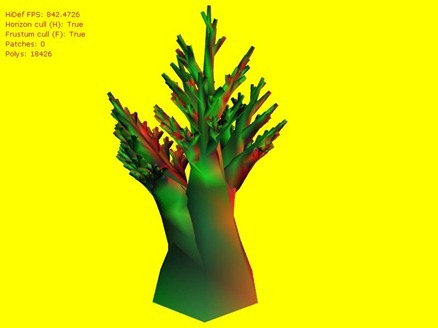
I continued working with the Algorithmic Beauty of Plants book and implemented parametric and context-sensitivity from chapter 1, made the trees from 3D tubes (instead of lines) and tried some of the examples from chapter 2 Modeling of trees. I had some success but couldn’t reproduce some of the models, mainly the section with tri-branching trees.

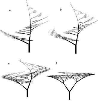
Here’s my results of the rules on page 56 varied with the parameters on page 57:

p56

And here’s what the original ones from the book look like:

p56original

They look pretty similar, apart from (b). Note that in (b) the height of my version is the same as the other trees, but in the book it is much shorter. This is odd because the table on page 57 modifies the branch contraction rate (r2) only, not the trunk contraction rate (r2) which is always 0.9 so they should all be the same height.

In fact, it’s not clear what the height should be to get the above images as the axiom at the start sets the length to 1 and the width to 10, and if the length:width ratio really were 1:10, the result would be a lot more squat, like this:

JellyEngineXna 2011-07-24 15-10-02-33

And it’s still pretty squat at 10:10:

JellyEngineXna 2011-07-24 15-10-26-57

I found a ratio of 100:10 worked best to yield results similar to the book.

The experiments on page 59 looked pretty much identical to the book (again using a ratio of 100:10 so an initial axiom of A(100,10) instead of A(1,10)), here’s mine:

p59

And here’s the books:

p59original

I had the least luck with reproducing the examples under Ternary branching. In the book (a) is shown as:

image

… which has a degree of irregularity… I don’t know where the model can get this as there is no stochasticity specified and the tropism applied is straight down (like the force of gravity), so why would the branch on the right bow down more than any other branch? My results show a much more regular model:

p60a

The closest of the ternary branching section I got was (b), although I had to fiddle with a few parameters (setting the width increase rate to 1.432 instead of the 1.732 given). Here’s the version in the book:

image

And here’s my result:

p60b vr1.432

(c) and (d) were real headaches… I can’t get these to look anything like the ones in the book… I’m pretty sure something’s missing ar the parameters specified are wrong, especially the elongation rate (lr) for (c); on page 61 it’s defined as 1.790 and all the others are 1.1 or less. Plugging this into my L-System/turtle interpreter results in a very tall tree (looking up at it in the first image and looking head on but zoomed out enough to see whole tree in the second):

JellyEngineXna 2011-07-24 15-38-40-99

JellyEngineXna 2011-07-24 15-39-01-39

I’m pretty sure my coding is right on this one, if you take the start piece from the axiom which is defined as F(200) and apply p2 (F(l) –> F(l*lr) 8 times with lr set to 1.790, this is the same as 200*(1.7908) which is about 21079. For the other trees, lr is 1.109 and the base trunk height after 8 iterations of p2 would be 200*(1.1098) which is about 457. However the image in the book shows the tree as the same height and roughly the same proportion to its width as the other examples:

image

If I muck about with the parameters a bit I can get something that looks a bit more like it:

JellyEngineXna 2011-07-24 15-47-56-31

… but it’s not quite as nice. (d) is the same story really, can’t reproduce it from the parameters given… :(

I’m *pretty* sure I’m right but this book has been out since 1990 and there’s nothing specified in the errata. I tried to find these models in the virtual lab available from algorithmicbotany.org but no luck. So I might fire off an email and see if any one associated with the book can help me out…

Other than that I implemented horizon culling on the planet with a lot of help from an article at crappy coding, redid some of my basic rotation stuff (I had everything mirrored through the z axis), and tried to streamline how new patches are formed on the planet (it didn’t work!). I’m not sure what to do next, had a look at some demoscene programs and am now utterly depressed at how little I’ve done! I might try generating normal maps from the heightmap of a planet patch for lighting, maybe do atmospheric scattering, texturing of the planet and/or trees, adding leaves maybe? Hiring someone else to do this for me?? :)

Tuesday, June 14, 2011

GPU Planet Update

Jeez, I can’t believe it’s been almost 2 years since I last did anything with this… I picked it up again a few weeks ago and tried to get into it again, made a little progress and thought I’d share.

A major problem getting back into it was migrating from XNA 3.1 to XNA 4 – there are lots and lots of changes, one of the worst I found was the restrictions placed on shaders and the Reach and HiDef profiles. I found an article which described how to target Reach and HiDef with the same project which was very handy, otherwise I’d have to develop 2 separate projects in parallel if I wanted to use both of my laptops for developing (one’s far more portable than the other but has to be Reach). So with a lot of help from this cheat sheet I got my project running again, and tried to learn a bit about shaders to see if I could get GPU noise back on shaders less than version 3_0_0.

In the process, I used a ping-pong technique to create Conway’s Game Of Life simulation (much better in 1080p):

The next stage then was to get back to the original goal of getting the GPU to generate all the noise as I found out doing noise in software was far too slow.

The plan was to pass the vertices to the shaders, let them calculate the noise then get back a heightmap which I can use to update the vertices. One of the problems was that the vertices form a curved surface and I need to flatten it for the pixel shader to give me back a regular heightmap. As each of my patches has texture coordinates that go from 0,0 to 1,1 I can create a flat image that the pixel shader could work with by using the texture coordinate to generate the position in clip space and storing the original position –which the shader will use to get the noise- in a texture coordinate. So for example, a point at 123, 234, 345 with texture coordinate 0.5,0.5 would end up in clip space at position 0,0 (clip space goes from –1 to 1) with the position stored as a texture coordinate. There’s a problem with halfpixel offsets as Drilian describes, in the end my shaders look something like this:

struct vertexInput {
float4 position : POSITION;
float2 texcoord : TEXCOORD;
};

struct vertexOutput {
float4 hPosition : POSITION;
float3 wPosition : TEXCOORD1;
};

float texel;
vertexOutput VS_flat(vertexInput IN)
{
vertexOutput OUT;
float clipx = 2 * IN.texcoord.x - 1;
float clipy = 2 * -IN.texcoord.y + 1;
float4 clipPosition = float4(clipx - texel, clipy + texel, 0, 1);
OUT.hPosition = clipPosition;

OUT.wPosition = IN.position.xyz;

return OUT;
}

float4 PS_noise(vertexOutput IN): COLOR
{
float3 p = 0;
p = IN.wPosition;
return inoise(p)*0.5+0.5;
}


And this technique let me create fBm on a 2_0_0 pixel shader by adding each stage of fBm in separate ping-pong passes:


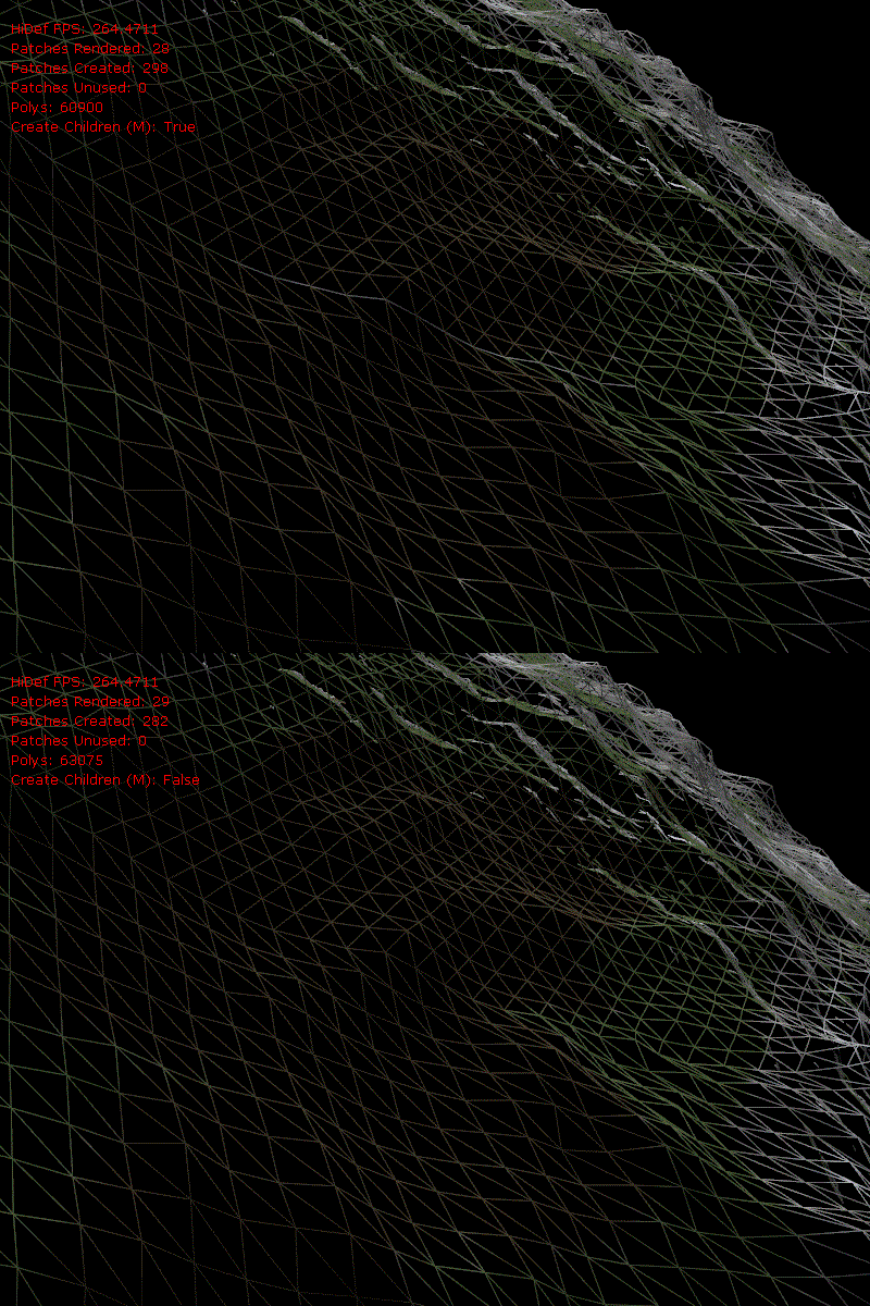
I used this in my original project and tried to update the vertices given the heightmap values generated by the shader. This didn’t work initially, I ended up with lots of cracks because of the way the pixel shader interpolates.


JellyEngineXna 2011-06-11 20-31-45-30


The upper left point (at tex coord 0,0) would have the correct noise value but I couldn’t get the lower right point to draw the correct noise value at tex coord 1,1. When 2 patches met they would have different height values for the same vertex. In the end I managed to get around it by rendering using a line-strip instead of a triangle-strip. This picture shows the same noise values along the edges of the patches:


JellyEngineXna 2011-06-14 10-47-12-57


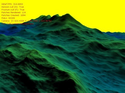
So, although it looks like I’ve made almost no progress since about 3 years ago (yikes!), I have! … made almost no progress that is :) The main difference is that this planet can render at run time – all the other planets had to have some pre-rendering of some sort, here’s a little fly around at 17x17 vertices per patch so you can see popping and subdividing:


In the end… it might be better to generate all the noise every time, for the vertices and for the pixels, caching the vertex info and texture is very heavy on memory. Hmm what’ll I work on next for an update in 2013…

Thursday, December 24, 2009

Blooming Starfields

It took AGES to add bloom. I used an XNA tutorial for bloom and in order to do the various passes (pick the brightest spots, blur it, recombine with the original image) it called ResolveBackBuffer to copy the back buffer to a texture for the next pass. I don’t fully understand it yet but it seems this call would invalidate the back buffer and subsequent shaders would write as if they were the first. I’ll try to illustrate what I mean by showing the problems I had. My plan was to draw the stars & clusters first, bloom that, then add the nebula.

Here’s what the result was like without the bloom stage, the nebula is added to the background stars (no bloom) as expected:

starfield without bloom

And here with the bloom stage included in the middle, it seems to be overwritten by the nebula stage:

nebula overwrites starfield with bloom In the end, I did a ResolveBackBuffer to a ResoveTarget2D after the bloom stage and drew this to the back buffer before I call the fBm/nebula shader. This finally ended in what I was looking for.

starfield with bloom

I’m still not 100% happy with the results, I had imagined the bloomed background stars would really light up the nebula but they seem to actually be dimmer than the stars outside of the nebula. I might try to use the same fBm noise result to draw some stars so they are in place in the densest parts of the nebula.

The main thing I’m not happy with though is that the code is a total mess, I just kept hacking and hacking away until I got results. I’m sure a team of monkeys would have produced neater code in less time. It’ll be a while before I get these images into a skybox – so until then HAPPY CHRISTMAS!